Quick Navigation
- 1Using Custom Number Formats in Excel
- 2Understanding the Number Format Codes
- 3Changing Font Color with Number Format Codes
- 4Adding Text with Number Format Codes
- 4.1Single Characters
- 4.2Text Strings
- 4.3Special Characters
- 5Changing Decimal Places, Significant Digits, and Commas
- 5.1Zero (0)
- 5.2Question Mark (?)
- 5.3Pound Sign (#)
- 5.4Period (.)
- 5.5Comma (,)
- 5.6Asterisk (*)
- 5.7Underscore (_)
- 6Using Fractions, Percentages, and Scientific Notation
- 6.1Fractions (/)
- 6.1.1Integer with Reduced Fractions
- 6.1.2Improper Fractions
- 6.1.3Fixed Base Fractions
- 6.2Percentages (%)
- 6.3Scientific Notation (E)
- 6.4Dates and Times
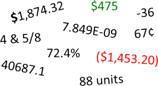 Excel has a lot of built-in number formats, but sometimes you need something specific. Whether you’re representing a little-used currency, tracking in-stock units, or want to color code profits and losses, you are in need of a an Excel custom number format. Number formatting in Excel is pretty powerful but that means it is also somewhat complex. This is the definitive guide to Excel’s custom number formats…
Using Custom Number Formats in Excel
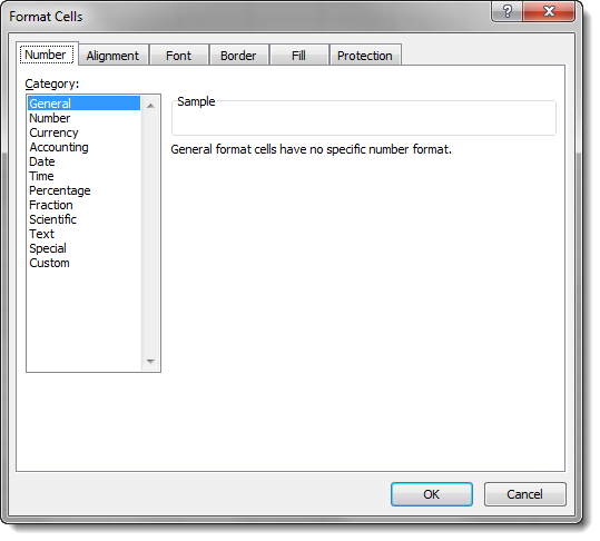
By default, each cell is formatted as “General”, which means it does not have any special formatting rules. When you enter data in a cell, Excel tries to guess what format it should have. When it doesn’t guess correctly, you need to change the format. Excel has a few pre-set formatting options attached to buttons in the Home menu, but if those don’t meet your needs, you need to use the full options available in the Format Cells menu.
To access this menu, look for the Number section of the Home menu tab. Click the arrow in the lower right corner of the Number section.
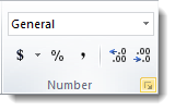
It will bring up the Format Cells menu in the Numbers tab:
Underneath the pre-defined number formats for common items like currency and percentage, there is a category called Custom. The format types in this section are different from the pre-set options. They are filled with symbols and codes:
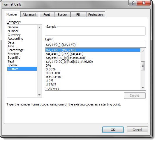
A number format code is entered into the Type field in the Custom category. These codes are the key to creating any custom number format in Excel. First, however, we need to understand how they work…
Understanding the Number Format Codes
Number format codes are the string of symbols that define how Excel displays the data you store in cells. We will get into the ways to describe the formats in a minute, but first we need to go over how Excel interprets those symbols. Each number format code is made up of as many as 4 sections separated by a semi-colon (;).
These sections control formatting for one or more parts of the number line, including positive numbers, negative numbers, and zeros. They can also control formatting for sub-sets of these parts, like all numbers greater than 100 and text-based data. What each section controls depends on how many sections there are in the number format code. A full number format code will be entered as follows:
Section1;Section2;Section3;Section4
The behavior of different parts of the number line will be as follows:
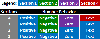
As indicated above, when there is just one section provided, it describes the format for all numbers. With two, the first section describes the format of positive, zero, and text values, while the second section describes the format of negative values, etc.
You can choose to skip formatting for any of the middle sections by entering General instead of other format data. For example, if you only want to affect positive numbers and text, you can enter a number format code with this arrangement:
Section1;General;General;Section4
General strips all formatting from the data entered, so be careful how you use it. Negative numbers with the General format code will not display the minus sign in front of their number.
Important note: Using a single section number format code does not always have the same result as expanding the same rules to all sections. For example:
Section1
Is not the same as:
Section1;Section1;Section1;Section1
Look at the examples below to see examples of the difference…
Now that we understand what a number format code is, what can we do with it?
Changing Font Color with Number Format Codes
One of the simplest things you can do with number format codes is change the color of the font in the affected cells. The syntax for doing so is simple:
[Color Name]
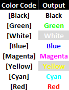
Just choose the section that corresponds to the part of the number line you want to change color, and provide the color in brackets. The color options are as follows (the background is gray for contrast in the table, but backgrounds are not affected by the number format code):
As an example, we can provide a separate color code for each part of a number format code:
[Red]General;[Blue]General;[Magenta]General;[Cyan]General
The General message just tells Excel to represent the numbers as entered by the user. The output of this number format code looks like this:
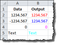
Note that the negative number in row 3 does not automatically get a negative sign (-) in front of it. We are overriding the default format of negative numbers in the cell. Also notice that the color format is not affecting anything about the presentation; the number of decimal places stays the same, as does the alignment of the data to the left or right of the cells.
Adding Text with Number Format Codes
You can add text around numbers with number format codes by inserting the text in a section one of two ways:
Single Characters
For single characters (like an @ symbol before a number), type a backslash (\) followed by the symbol. The number format code:
\@General
Results in the following output:
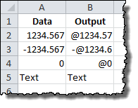
Note that the minus sign still precedes the negative number. Also note that the Text value is not affected by the @ symbol addition.
Importantly, this is different from the result if we expanded our format guideline to each section of the number format code:
\@General;\@General;\@General;\@General
Results in the following output:
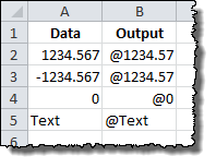
Note that the minus sign is gone from the negative number and the Text value now receives the @ symbol.
Text Strings
To add an entire text string to a number (like adding “units” to the end of a number), we surround the text string in quotation marks (” “). The number format code:
General" units"
Results in the following output:
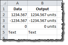
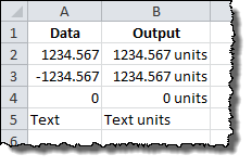
Once again, this is different from:
General" units";General" units";General" units";General" units"
Which results in:
Special Characters
In addition to these two methods, there is a set of special symbol characters that do not need a leading backslash or quotes to be included in the number format code. The list is as follows:
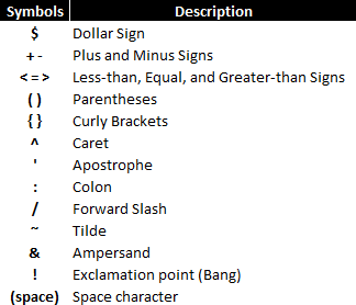
Excel will also accept most other non-mathematical symbols, such a non-dollar currency symbols, copyright/trademark symbols, and Greek letters. These symbols are not available on most standard keyboards, but they can be entered by holding down the ALT key while typing in a four-digit number. Some of the most useful ones are below:
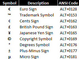
A full list of ANSI character codes can be found on Wikipedia here.
Changing Decimal Places, Significant Digits, and Commas
Adding symbols and colors is useful, but most of the work you’ll likely need to do with custom number formats is change the way Excel displays the numbers it stores. Number format codes use a set of symbols to represent how the data should appear in the cell. Here is a summary of the symbols:
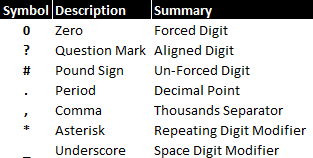
Let’s review them each in turn…
Zero (0)
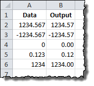
Zeros in the number format code represent a forced digit. That means that whether or not the digit is relevant to the value, it will be shown. A great example of this is the standard dollars and cents notation that is used to represent prices in the United States: $0.00. Even if there are no extra cents in the amount, the two zeroes are still shown in the notation.
Here is an example of the zero code in action. The following examples are using this number format code:
0.00
Question Mark (?)
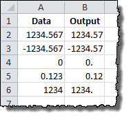
Question marks in the number format code represent an alignment digit. This means that when the number being shown doesn’t need the digit in question, a blank space of the same size is used. This is used to align decimal and comma places for more easy ranking of values, etc.
Here is an example of the question mark code in action. The following examples are using this number format code:
0.??
Pound Sign (#)
Sometimes called a hash mark, the pound sign in the number format code represents an optional digit. This means that when the number being shown doesn’t need the digit in question, it will be omitted from the displayed number. This is most often used to represent numbers in their most easily readable form.
Here is an example of the pound sign code in action. The following examples are using this number format code:
#.##
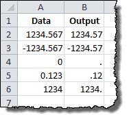
Period (.)
The period in the number format code represents the location of the decimal point in the number being displayed. When paired with the comma code, it can show numbers in thousands or millions, changing 1,200 to 1.2, for example. It is similar to the text format codes above in that it is always displayed when it is part of the number code, even when number being displayed does not straddle the decimal point. See the comma, pound sign and question mark examples above for useful illustrations of the period in use.
Comma (,)
The comma in the number format code represents the thousands separators in the number being displayed. It allows you to describe the behavior of digits in relation to the thousands or millions digits.
Here is an example of the comma code in action. The following examples are using this number format code:
$??,???.00
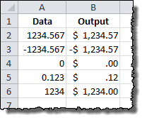
Asterisk (*)
The asterisk in the number format code represents the repeating character modifier. It is used along with a character to display a repeating digit that fills the empty space in a cell.
Here is an example of the asterisk code in action. The following examples are using this number format code:
*=0.##
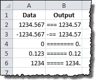
Underscore (_)
The underscore in the number code represents the space character modifier. It is used along with a character to display a blank space equal in size to the specified character. It can be used, for example, to properly align positive and negative numbers when parentheses are used in only the negative case.
Here is an example of the underscore code in action. The following examples are using this number format code:
_(#.##_);(#.##)
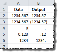
Using Fractions, Percentages, and Scientific Notation
Certain types of notation require that symbols be used to indicate the format change, including fractions, percentages, and scientific notation. Here is a summary of the symbols for each:

We’ll examine each in detail…
Fractions (/)
Fractions are special, since they require a change in units. The number 0.23 is represented as 23/100, but 0.25 can be simplified t0 1/4 or shown as 25/100. Similarly, 1.25 can be shown as 1 1/4 or the improper fraction 5/4. Which way Excel displays the number depends on how you construct the number format code.
Fractions effectively round values to the nearest possible fraction. They also take the guidelines of the pound sign and question mark symbols they are paired with.
Integer with Reduced Fractions
A fairly typical representation for fractions is to keep the whole numbers independent from the fraction remainder. The representation for this is relatively straightforward and can be done with pound signs and question marks to slightly different effect…
Using question mark (?) notation, the following number format code:
# ???/???
Produces a fraction remainder with up to three digits:
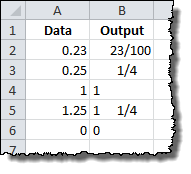
The alignment of the fraction bar is preserved regardless of the number of digits in use. If we limit the number of digits on each side of the fraction to 2, Excel will round the number to the nearest fraction value. The following number code format:
# ??/??
Changes the representation of 0.23 from 23/100 to 3/13.
If you don’t wish to preserve the alignment around the fraction bar, you can use a similar fraction number format code that uses pound signs.
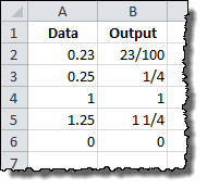
Using pound sign notation, the following number format code:
# ###/###
Produces a more readable fraction remainder that can be justified or centered in the cell:
Improper Fractions
If you’d rather bundle the whole number portion of a value into the fraction itself, you can specify as much in the number format code.
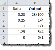
Using pound sign notation, the following number format code:
###/###
Produces an improper fraction with up to three digits:
Fixed Base Fractions
It is also possible to force Excel to round fractions to a specific denominator by specifying it in the number format code.
Here is an example of a fixed base code in action. The following examples are using this number format code:
# ##/15
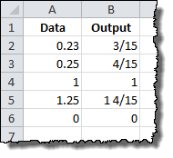
The result is a rounded fraction remainder that goes to the nearest number of 15ths.
Percentages (%)
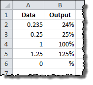
Much like fractions, percentages are controlled by the number format codes that accompany them. A basic percentage can be achieved with a pound sign symbol in the number format code:
#%
Results in the following output:
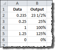
You can also specify fractional percentages, as shown with this number format code:
# #/#%
Results in single-digit fractions in the percentages where needed:
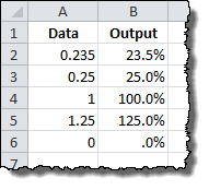
Finally, as always, you can specify the number of significant digits with decimal places:
#.0%
Results in a 10th place aligned decimal:
Scientific Notation (E)
It’s difficult to read extremely small and extremely large numbers conventionally because of all the leading and trailing zeroes. Scientific notation fixes that by moving the decimal to the relevant digits, so 0.0000001 can become 1 x 10⁻⁷. Excel uses the E notation for this, so that same number would be 1E-07. So, as you’d expect, the capital letter E signals scientific notation in number format code.
Otherwise, scientific notation in Excel is controlled by the same number codes as percentages and fractions. It needs a number format code in front of the E to describe the relevant digits and a plus (+) and another number format code behind to describe the handling of the exponential digit.
Here is an example of a scientific notation code in action. The following examples are using this number format code:
#E+#
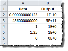
You can also achieve more consistent notation with zeros. The following examples are using this number format code:
0.00E+00
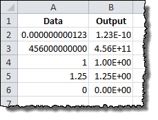
Note that in this case, the decimal and exponent are both constrained to 2 significant digits, regardless of whether they are necessary. The trade-off is, it keeps the output far more consistent, with a predictable string length.
Dates and Times
Dates and times in Excel are a special case. For a detailed discussion of how Excel uses them, please review the Definitive Guide to Using Dates and Times in Excel. The number format codes work identically to the format_text input for the TEXT command, and they can be reviewed here.
Pretty nice exhaustive article. Thanks man! Subscribed to your list.
I have a column of numbers that have varying numbers of decimals characters. I need to only show the digits. Is there an easy way to only show the numbers without the decimal?
Thanks!
Hi,
You can simple do this by selecting the cells, choosing format, number and then use the “Decimal Places” box to select 0. This will make excel automatically format each cell by rounding up. So bear that in mind 🙂
Also – good article, thanks for info.
Oh!! That one is an easy one.
I’ll assume that all numbers are positive and that some may be in the thousands.
Use the following format:
#,##0
That’s it. If you have some negative numbers in that list you may use:
#,##0;(#,##0)
Pos Neg
Hummm! Let’s see. How about using the “Decrease Decimal” button in the Ribbon.
Select all the numbers then click “Decrease Decimal” as required.
If you want to know more about “formatting-a-negative-number-with-parentheses”, check this link ……..
http://www.exceltip.com/excel-format/formatting-a-negative-number-with-parentheses.html
I am trying to force a Code 39 Bar Code in a 00000-0000-000 (5-4-3) format.
What is wrong with my syntax:
“*”(00000)”-“(0000)”-“(000)”*”
Thank you!
I am using Excel 2013 and the format 00000″-“0000”-“000 works. Any extra digits are added to the 5 digit segment; less than 12 digits results in lead zeros.
Format code below works for me:
(00000)-(0000)-(000)
There is also Engineering Notation, a sub-set of Scientific Notation. I displays numbers in an exponential-3 format:
Engineering Notation
Engineering Notation uses a format similar to Scientific Notation, but its exponents are always expressed in powers of three. Consequently, the mantissa is expressed as n = 1.000… to 999.999… . The usefulness of Engineering Notation is that it readily makes evident the number of thousands (103 or kilo), millions (106 or Mega), billions (109 or Giga), thousandths (10-3 or milli), millionths (10-6 or micro), billionths (10-9 or nano), etc., of a numerical value.
The following format causes numbers to be expressed in standard Engineering Notation, with three places after the decimal and two digits (with a leading zero) in the exponent:
Format Example
###.000E+00 299.792E+06
The following format causes numbers to be expressed in standard Engineering Notation, with up to nine places after the decimal:
Format Example
###.#########E+00 8.854187817E-12
Note: To cause whole numbers to have at least one digit after the decimal point, place a zero (0) immediately after the decimal point in the format code:
Format Example
###.0########E+00 400.0E+03
The following format causes numbers to be expressed in standard Engineering Notation, with at least three places and up to three additional places after the decimal:
Format Example
###.000###E+00 400.000E+03
The following format causes numbers to be expressed in standard Engineering Notation, as above, but with a space between the “E” and the last digit of the mantissa:
Format Example
###.000### E+00 299.792458 E+06
The following statement causes values in kilowatts less than 1000 to be displayed in a format with trailing zeros or tenths of kilowatts shown, and values in kilowatts greater than or equal to 1000 to be displayed in a format with trailing zeros omitted or tenths of kilowatts rounded up to the next kilowatt:
[>=1000]#,##0.#” kW”;[<1000]0.0" kW"
Engineering Notation is mostly used by electrical and electronics engineers, and in those engineering colleges and universities where courses in those disciplines are taught.
Thanks Charles! That Engineering notation is exactly what I wanted for custom notation. Thank you.
I constantly work with long, 16-digit claim numbers that are numeric. We need them to show all 16 digits, but copying a column of them into Excel puts it in Sci Notation, and even converting from that to “Number” will round off the last few digits, which is not acceptable. Formatting the column as “Number” before pasting causes the same result. How can we get Excel to recognize the full number without loss of information?
I’m trying to sort data using a column that contains codes with three letters and four numbers such as AAA1212. When I sort, the custom mmm-yy format built into the ss converts some of the codes – the ones with APR or AUG for example, into date format such as APR-12. Changing the format to text or general produces a result that is a string of numbers, eg 1612301. What format can we use in the column keep the original data of AAA1212 or AUG1212 when so we can sort the sheet by the column with this data?
I work with Bond quotes that are in 32nds. This is understood throughout the industry so it’s common to drop the 32 from the fraction. 102 10/32 would be displayed as 102 – 10 (also much faster to key in on a 10-key). Any idea how I can accomplish this with cell format?
Does the cell that the data is keyed into have to recognized as 102.3125?
Can the display cell be a different cell from the data entry cell?
Can the whole dollar value and the fractional value be in different cells?
Finally, does or can your spreadsheet have some VBA embedded?
I am trying to format cells as “GENERAL” with comma separators – 12,313; 2.387; and 1,287.5694 would display exactly as I typed them here. The closest I have come is a format that will display the decimal point whether or not there is anything after it – 3 is displayed as “3.” Any suggestions?
I have the same issue and utilize the MOD function. Here’s a sample:
TEXT(E87,IF(MOD(E87,1)0,”#,##0.0#######”,”#,###”))
I’m converting source data so I stick with the excel function. I’m sure you could use VBA if the data entry cell needs reformatted.
You could do a conditional format. So the normal custom format is: #,##0.#### or whatever. And then add a conditional format (Rule type: Use a formula), formula is =mod(A1,1)=0 , and format if this is true is: #,##0 or similar, where A1 is the upper left cell in your range.
I can uses little help
I have cell that Number is entered as 2,4 and I like to uses Custom cell format to end up with CKT 2,4
is this possible? the comma is the entry is giving me problems “CKT” “”# if no comma ends up with CKT 24
Use the following custom format:
General;General;General;”CKT “General
It will treat numerical values and zeroes in the usual “general” manner. (You can change any of the first three elements to make each one more what you’d like.) The fourth part though, is telling it how to format text entries. Since something like “2,4” is a text entry this is the portion you need to adjust, NOT the first two parts.
The key again, is that something like “2,4” is text, not numerical (for anyone named Howard… probably… and if not because the comma is a decimal separator, it would have already been handled so…). Therefore the place to affect its format is the FOURTH portion of the custom format.
You may want to give this one a go:
;;;”CKT “@
The three ; are not used as they are dedicated to numbers. the @ is for text (if you add a numeric value it will be converted to text.
I used the format above then simply type 2,4 then Enter to get: CKT 2,4
2nd question
can the tab sheet be linked to a cell on other sheet
so if Sheet2!B44 was” Dinner” then sheet tab on disired sheet would show up as Dinner
Of course, VBA can do almost anything one asks for, but outside of VBA, there is no way to do this.
Sheet names CANNOT be changed except via human or VBA entry. No formula or setting can do it. So NO, there is absolutely no way for this to happen without typing or VBA.
Going the opposite direction can be done. (Using a formula to learn the sheet name and using the result in the rest of the formula to put a value in the cell.) People need to do so reasonably often. But it cannot go from cell to sheet name, only sheet name to cell.
Nice find, your site.
I’ve been working on inserting non-printing control characters in custom formatting: “^p”, for instance, to produce a line feed. Custom formatting doesn’t seem to accept the above or a keyboard entry: Alt+return.
So far I’ve been reduced to constructing concatenated TEXT() functions.
Am I missing something?
JMarks.
Hi friends,
I was trying to format a cell with similar to following manner, where the engineering notation has to star with 0.. Any suggestions?
1.751200E+12 => 0.175120E+13
You forgot to mention additional uses of brackets in Excel custom number formats. You can use brackets for conditional formatting using a custom number format, rather than using Excel’s Conditional Format feature (which while allowing more options, is also more cumbersome to code in some scenarios).
Example custom format: [=1] 0 “cup”;# ?/? “cups”
If the cell value is equal to 1, the contents will display as: 1 cup
If the cell value is equal to 2.5, the contents will display as: 2 1/2 cups
As you can see, depending on the value of the cell we want to use different text and number formatting.
I find this feature extremely useful, though rarely used. Unfortunately very few (if any) websites discussing Excel custom formatting cover this feature (if at all). To be honest I couldn’t find any websites discussing this feature, and was only able to use it / discover it through trial and error, though I stumbled across it years ago in an Excel developer forum.
How far you can go with this particular feature I really don’t know, but the possibilities are very intriguing. I do know you can also use much more complicated variations like example format: [=3] 0 “more”; 0
and when the cell value is equal to 1, contents display as:
1 less
when the cell value is equal to 3, cell contents display as:
3 more
and when the cell value is equal to 2, cell contents display as:
2
Proving that conditions in brackets can be combined.
As I said, this little know feature is very interesting, but I really wish someone could expand on this and define the rules governing this feature of custom number formats, and it’s limitations.
Many websites address exactly this. They usually don’t make much of a point that you have the choice of using the (up to) four portions available for EITHER:
positive #’s ; negative #’s ; 0’s ; text entries
OR
Condition 1 ; Condition 2 ; Condition 3 ; Condition 4
but CANNOT mix and match the approaches. So you cannot use the first two for condition tests, and then the final two for 0’s and text entries. Small point but it matters sometimes.
Also, the conditions can be “combined” in the sense of using (up to) four of them, but you cannot put two or more conditions in ONE of the formatting string’s portions. Each condition takes one of the four portions.
But quite so. Very handy for taking the burden off solving the display issues you face in the cell’s formula which usually greatly complicates said formulas. Also a nifty way of hiding some of the spreadsheet’s logic if that matters to an organization. Another useful aspect is that doing this takes a burden off what would otherwise be very complicated conditional formatting and might make something that couldn’t be done with CF into something possible, even easy.
All that said: Like anything, it can’t fix everything.™ So often it cannot help or would make it harder instead.
Like Mr. Callaghan says, very handy. If you remember about it!
(Just kidding about the ” ™ ” thing up there. Still though…)
It is truly helpful, especially to display Indian numbers, where commas are placed at thousandth, 100 thousandth, 10 millionth, 1000 millionth and 10 billionth places. Surely only a part of it can be formatted using square brackets. But that itself is a big relief for personal accounting worksheets.
I am trying to display 15 numbers to the left of the decimal and 4 to the right. I am using ##############0.0###; however, it appears the cell will not display more than a total of 15 digits. When I have 4 digits after the decimal, to make sure they all get displayed, the most digits I can have to the left of the decimal is 11. For each digit I add to the left past 11, I lose a digit to the right of the decimal. Is there a way to display all 19 digits?
Use two cells on the same row; in the left cell, use [FORMAT CELL], [NUMBER], (Decimal Places) – 0 (zero), and in the right cell, use [FORMAT CELL], [CUSTOM], (Format) #.0000.
Then, divide the number you want to display into an integer part & a fractional-decimal part.
Hi
When I enter say 23 I want the default display to show 23.00 but at present Excel shows 0.23.
I cannot find a way to set up all of my spread sheets with this default format and then all I have to do is selectively change the minority of other formats, dates, etc as and when I need to
I think your Excel Setting “Fixed Decimal Points” might be on and set to 2. Try looking for it in the Options. If taht is the case, in order for Excel to display 23.00, you have to enter 2300.
Thank you that solves the problem
Wrong; this setting can be changed:
Click the OFFICE BUTTON at the top left corner of an Excel page; select EXCEL OPTIONS (at the bottom of the page); select ADVANCED; then under EDITING OPTIONS, check or uncheck AUTOMATICALLY ENTER A DECIMAL POINT; then click OK at the bottom right of the panel – if checked, entries apear in hundredths, if unchecked, entries apear as whole numbers; finit.
Click the OFFICE BUTTON at the top left corner of an Excel page; select EXCEL OPTIONS (at the bottom of the page); select ADVANCED; then under EDITING OPTIONS, check or uncheck AUTOMATICALLY ENTER A DECIMAL POINT; then click OK at the bottom right of the panel – if checked, entries apear in hundredths, if unchecked, entries apear as whole numbers; finit.
Great article, but I have a head scratching problem. I need to show 2.50 as 000250, any idea on how to do that without using a text format?
format with custom: 000000
will add leading zeroes
Hi.
Is there a way to save custom format cell. Facing problem when doing same thing in another file, it disappear automatically in next file
For your reference Image is attached.
Regards
Sat
Custom formats are saved with the files they are created in. The only way to carry over formats would be to adjust your PERSONAL.XLB file, but these might not transfer to other computers and that is beyond the scope of this article. Good luck!
I want to format cell that displays date and OPTIONALLY time. Meaning, when the time exists, display it but when it doesn’t, HIDE it (don’t display 00:00).
You will need to use two separate cells to do it this way:
For two adjacent cells:
(1) Place the date-time value in the first cell.
(2) Place =[CELLNAME1] in the next cell over, or down; whichever way you want it displayed
(3) Format the first cell in whatever Date format you want.
(4) Use Conditional Formatting to format the second cell with this statement:
=AND(HOUR(CELLNAME2)=0,MINUTE(CELLNAME2)=0,SECOND(CELLNAME2)=0)
(5) Specify WHITE as the font color if the above condition is met.
The first cell will display the date, and the second cell will display the time if the time is non-zero.
This is the best Custom Format article I have found
Thank you very much
And also thank you Charles for the Engineering and Electrical notation examples. Very helpful.
Cheers,
Ben
Dear Sir,
I want to use this custom numbers format in excel permanently.
[>=10000000]##\,##\,##\,##0;[>=100000]##\,##\,##0;##,##0
when i adding in customs formats , after closing of workbook it will not working.
kindly advise permanent solution.
Custom formats are stored by Excel; so they will still exist after closing, then opening a workbook; but the format must be invoked for each cell or set of cells in which you want to display the format, and that workbook will need to be saved, as well. To transfer a format to other cells, you can use the “Format painter” feature (the icon is a paintbrush), or merely copy or cut the cell into another cell. Additionally, this format is also one of the standard formats available in Excel. You can select “Format Cells”, “Number”, click the DOWN or UP arrow in the “Decimal Places” box until the number in the box is 0 (Zero), & check the “Use 1000 Separator (,)” box. This format will also still exist after closing, then opening a workbook; but you will need to invoke it for each cell to which you want it applied.
I have columns of over 50,000 numbers ranging from 2500 to 0.000021. I am given the numbers in an excel spreadsheet with 9 decimal places. I need to change the decimal place format to the lowest number, as in 1.5, 0.02 and 0.505 instead of 1.500000000, 0.020000000, and 0.505000000. I used to be able to do this using advanced find/replace and wild cards, but I have forgotten. Any ideas?
Yes; use “Conditional Formatting” – “New Rule” – “Use a formula to determine which cells to format” under the “Home” tab, & set up different formats for numbers based on their values, then apply the format to cells as needed.
When I enter a formula in Excel it appears automatically as an absolute reference. How can I get it to default to a relative reference?
I WANT TO CHANGE THIS TYPE OF NUMBER AT A GLANCE
+1(942) 266-3741 CHANGE TO 9422663741
Place your number string in a cell; in this example, cell B19. Then in another cell, place this command: =MID(B19,FIND(“(“,B19,1)+1,3)&MID(B19,FIND(” “,B19,1)+1,3)&MID(B19,FIND(“-“,B19,1)+1,4). The cell will then display your number as you want it.
I have text-type content of a cell, for instance: “123ABC456”, is there any way to use Custom Format to get in result “123 ABC 456” (formatting should add spaces before and after actual text – separate it from digits)?
Unfortunately, no – formatting can only change the way data in a cell is displayed. To add spaces, you would need to use formulas to calculate the change.
No: however, you can get Excel to display your characters the way you want by placing the character string in a cell, in this example, cell A4; then in the next cell to the right, enter “=LEFT(A4,3)” with a cell width of 2.83; leave a blank cell with a width of 1; in the next cell to the right, enter “=MID(A4,4,3)” with a width of 2.83; leave another blank cell with a width of 1; and finally, enter “=RIGHT(A4,3)” in the last cell.
Oh, I forgot to mention that the last cell needs to have a width of 2.83, and that the left-most display cell needs to have a left-align applied to it, the center-most display cell needs to have a center-align, & the right-most display cell needs to have a right-align.
The problem is that I would like to avoid using another cell/column to get the result, and maintain original value (spaces are only for user convenience). What’s more, it’s not necessary to use 5 additional cells/columns – it could be done using one formula in one cell (just join your three formulas using &” “&). Anyway, thank you for your effort!
Yes, that does work.
custom formats won’t do it try one of these, they’re equivalent.
=CONCATENATE(LEFT(A1,3),” “,MID(A1,4,3),” “,RIGHT(A1,3))
or
=LEFT(A1,3)&” “&MID(A1,4,3)&” “&RIGHT(A1,3)
Great article! The only thing I don’t see is information about the @ character. As best I can tell, that code tells Excel to treat the value as text. So @*. creates trailing periods, which is awesome! Unfortunately, using the @ code appears to remove any other formatting, so the superscript portion of a cell (used to denote a footnote) gets stripped of the superscript and shown as standard text. Bummer!
I am not sure how to format WITHOUT adding spaces in the a cell from “1234567890R1” to “12345 67890 R1”. Would someone know how to do the formatting code? Thank you.
Hi Catherine! The example you provided has numbers and letters, so Excel won’t treat it as a number field. You can add spaces by using LEFT(), MID(), and RIGHT() to break up the field.
Hi
I have lots of numbers in millions – is there any way to make the comma (thousands separator line up so the relative digits align
Use a Currency format, or similar Custom format in the cells, & impose Right-Alignment on those cells.
I have a negative number in a cell, like -1.232 , and I want to use custom format cell to make it look like B=-1.232, but when I type “B=” #.### the minus sign goes in front of B like -B=1.232. Can somebody help? Thanks 🙂
Charles gives an answer that is working overly much.
You DO need to enter something for the first portion (positive numbers), follow it with a simi-colon, and then lay out your format for the negative numbers. Otherwise Excel reads the format as applying to all values. Worse though, since it would seem like that would still let the negative numbers be displayed correctly (!), the “-” is a special character to this functionality and Excel sees it as more text (the very same, to it, as the “B=” in the parentheses) and it puts the TEXT “-” in after the “B=”… that “-” is NOT the negative sign in this display. The “-” out front IS. However, once you enter a string (just the word General will be fine) for the positive value portion, and push this formatting into what it realizes is just for negative values, it also knows you may want to specify a location for a “-” and does NOT treat the one in the string as text. So it now knows you want a negative sign right after the equals sign. So you get the desired result.
Where Charles overworks is that you do NOT need to enter anything for the third and fourth portions. They are fine being empty as far as Excel is concerned.
(It doesn’t truly care about the first portion being specified. It’s just that there is no other way to make Excel realize the format you DO want to specify is for the negative values ONLY. So you have to specify something there, even if just “General” to make that realization come to Excel.)
Excel uses four format code sections; format for positive numbers, format for negative numbers, format for zeros, format for text.
To get the displayed result you want, use the following format string:
“B = “0.000;”B = “- 0.000;”B = “0.000
or
“B = “0.000;”B = “- 0.000.
If you don’t want the spaces between the characters, eliminate them.
I have a column of numbers example 345. I need to only show the last digits 5. Is there an easy way?
Thanks!
In a cell, place your multi-digit numbers; in the next cell over, use the RIGHT text function:
=RIGHT([cell],1), with [cell] being the cell reference.
The result will look like this:
345 5
692 2
157 7
468 8
For international readers: if your system is using “,” (comma) as decimal separator, you have to mentally exchange , and . when reading this article. For example, in Latvia we use to format currency values like this:
# ##0,00##
which results in
1 234,56
1 234,00
1 234,5678
Great information, the engineering notation especially useful for me. Any suggestions how to format a complex number? They always display with full decimal places, e.g. 1.65287436333954+1.34696283284023i
There are two ways to build complex numbers in Excel:
(1) place the real and imaginary values in separate cells and use the COMPLEX function.
(2) enter the number directly, as in 1.65287436333954 + 1.34696283284023i.
Excel treats both equally with respect to the complex number functions.
If you want numbers rounded off, use the ROUND function embedded within other functions, as in =COMPLEX(ROUND([CELL],3),ROUND([CELL],3)), or
=ROUND(A205,3)&”+”&ROUND(B205,3)&”i”
Excel also treats both equally with respect to the complex number functions.
Addendum:
I you want to have spaces in the built-up version with the ROUND function, use =ROUND(A205,3)&” + “&ROUND(B205,3)&”i”
Hi guys. I’m working on a spreadsheet where I’m using 1 row per ‘item’ and so I’m trying to get some cleaver formatting into a particular cell. Under the heading of File Location, I’d like to put the ‘name’ of the location and the ‘path’ but aligned in different directions, ie:
———–File Location—————
Workspace
C:\MyWorkSpace\
___________________________
Workgroup
C:\
So I’ve been trying to use the repeat character formatter “* ” to align the 2nd line of text to the right. However this only really works for a single line of text per cell. If the cell contains the text “Workspace” and the number formatter contains the text “@* “C:\MyWorkSpace” and the cell is wide enough, then everything looks good. But put a newline character in (Alt+Enter) after the word Workspace, then you’ll see that the 2nd line doesn’t align to the right properly. Can anyone think of a fix for this?
You can do this IF:
1) You just have two lines. (It looks like you do, just have two examples.)
2) Have only one place where a “space” character has to go.
(#2 can be cheated if you are able/willing to use whitespace characters that are NOT the keyboard “space” character for all other places the “space” character exists.)
Use a cell format called “Distributed (Indent)” (found on the Alignment tab in formatting for Horizontal alignment).
In its simplest form, this pictures, say, “horse pig” being entered and it will separate them using that space putting the “horse” part at the extreme left of the cell and the “pig” part at the right edge. More words, and therefore spaces? It divides the contents into that many pieces and more or less splits the whitespace in the cell evenly between each piece.
That last is why your use here must not have extra “spaces” though it is perfectly happy if you use other whitespace characters where you want extra spaces.
Further complicating your need though is that in a simple use, the single space between horse and pig is enough for it to be happy as it seems happy to regard that space as BOTH following horse AND as separately preceding pig. Huh? Clear in a second…
With the use of Alt-Enter though, it cannot regard a single space after horse/before pig as part of both portions. The Alt-Enter breaks that idea. So you need to put a space after horse, then Alt-Enter, then another space to precede pig and it’s all good. That oddity, that there must be a space for it to hang its shingle on must be paid attention to.
And then you have exactly what you want.
(If either line does not have its space, it centers the contents. There are some other not so easily predicted effects if you add other spaces, more separate portions, like “horse cow pig” perhaps. Might be some that are useful to.)
A common use of this formatting is a label that must label something to its left and something to its right. A breaker box maybe or a file folder label that shows the starting contents on the left and the ending contents on the right.
I want to use the “Single Accounting Underline” with a custom format with percentages but I cannot get this to work. It only underlines the number.
Surprised not to see any mention of the other use of the comma. Adding a comma at the end of the formatting code rounds the value to the nearest thousand. Adding two commas rounds to the nearest million. Thus using a format code of “#,##0.0,” the number 12589 is shown as 12.6 and 23 is shown as 0.0. Similarly, using a format code “#,##0.0,,” 123456789 is shown as 123.5
How do I reverse that? If I have 3,604 and want to change it to 3,604,000
Every now and then, I find a post the EXACTLY answers my question in a clear, concise, accurate and complete manner.
Thanks for that.
Hi – I somehow stumbled on this website that “FINALLY” explains a lot that I’ve been desperately looking for. However, I am still struggling to find a simple solution for displaying both positive and negative-red-values for the Indian Rupee.
For positive numbers, this works:
[>=10000000][$INR] * ##\,##\,##\,##0.00;[>=100000][$INR] * ##\,##\,##0.00;[$INR] * ##,##0.00
For negative numbers, this works:
[Red][<=-10000000][$INR] * -##\,##\,##\,##0.00;[Red][<=-100000][$INR] * -##\,##\,##0.00;[Red][$INR] * -##,##0.00
But how do I combine the two ? Combining them with a semicolon does not work – and I now understand about the 4 section bit.
Is it possible to group the positive and negative formatting in parenthesis ? Is there another option available ? I will be very grateful for a solution to this.
Thanks
Also looking for a way to combine two conditions/formats for positive/negative numbers. Personally just want to display numbers >= 1000 and <=-1000 with a comma and no decimals, and anything else with two decimals. Help would be appreciated!
Hi Alaina. Interested to know whether you ever found a solution?
How can I get the following format #:# (i.e., single integer colon single integer)?
Use: #”:”#
But bear in mind that it is STILL the number typed. So enter “45” and while it will display as “4:5” it will still be decimal number 45 and dividing it by 15 will result in 3.
(To get it to NOT do that, although it is hard to see why you would need to, use a helper column with the TEXT() function and that as the output format… except that since the format there has to be IN double quotes, the double quotes in the format string above have to have an extra double quote by each one so: “”:”” instead of “:”…)
Excellent comprehensive article! Thank you.
Quick question, is there a way to format data tables within Excel?
Thanks again for posting this.
Thank you for the article!! Very helpful! Ive got an issue I can’t seem to resolve. is this possible?
I’ve got a format that changes from this:
22-22-222 to this: 22-2a-222 to this: 22-aa-2222 randomly throughout column E of my worksheet. It changes back and forth between the above mentioned formats.
Is there a custom format I can implement so that it will stay the same all the way down the entire column?
Thank You In advance!
Hi. I want to display a number, say, 20 in format “at 20°C”. I make Custom Formatting as “at “#”°C”, and it shows what I want if the temperature is positive. When it is negative I see “-at 20°C”. Please help.
Thank you.
Regarding colors: you are not limited to those listed.
I wanted to make grey text, tried using the color names with numbers such as Color48 (they range from 1 to 57, you can find many references by googling “excel number format color numbers”).
Let say I have two numbers, 10% and 10.5%. Is there a way to format the number so that the since the 10% has no fraction, there will be no decimal point, but since 10.5% has a fractional percentage, that will be shown. Thank you!
This information is fantastic! Thank you!! I’m looking for suggestions on how to format a cell with a particular format. Here’s an example:
How it’s keyed into worksheet: 20170215021KC
Need to autoformat and display as: 20170215_021_KC
Any suggestions will be greatly appreciated.
Lower to upper case in the same cell (custom format string) i.e. cell A1 = n (change to upper case) cell A1 = N (how to custom format string)
My custom added numbering disappeared after closing and reopen the excel. Anyway to resolve it?
Hi Ryo! Custom number formats are saved in the spreadsheet you worked on when adding them. If you want them to load every time, you need to save them in the startup template Excel uses when it loads. Search for “Excel Startup Template” or go here for more details.
Hi Andrew,
Solved! Thanks a lot!!!
It’s pretty hard to me. 😀 Anyone could tell me what kind of code I need, if I want to display 0 as 00/00? For 1 it’s 00/01, for 10 it’s 00/10, for 100 it’s 01/00, for 1000 it’s 10/00, for 10000 it’s 100/00 etc.
00\/00
That will display the numbers as you wanted to . But note that for example 2344.3455 or – 67 will be displayed as 23/43 or -00/67 respectively.
I am trying to format phone numbers that may or may not have an extension. If the number has an extension, the extension may be 1-5 digits long. If there is an extension I want to display an “x” after the 10 digit number followed by the extension. So, if the cell value is 123555121299887, I want it displayed as: (123)555-1212 x99887.
And a cell value of 234555121298 should display as (234)555-1212 x98
I tried this custom format: [<=9999999999](###)###-####;(###)###-#### x#####
but it only works for numbers w/o an extension and those with a 5 digit extension. For extensions with only 1-4 digits, the cell value gets displayed from the right to fill up the 5 extension digits first resulting in the area code portion & phone number getting messed up.
So a cell value of 234555121298 is being displayed incorrectly as ()234-5551 x21298
I don't want to use a multi-column solution, just 1 column for the phone numbers.
Hi – I’m trying to sum cells which use a custom format to display “Kb”, “Mb”, “Gb” but I can’t find how to determine the Custom Format so I can add say 3 cells containing 23 Mb, 15 Mb and 230 Kb to display them in a common form say 38.xxx Mb. Any thoughts ?
hi
i want to make a colomn witch shows number like this:
12.3 ==== 12.3
0.3 ==== 0.3
5 ==== 5 (when i use ?.??? it ads space(3 spaces after 5) and and shows 5. that is not desirable)
thanks for your attention
Can excel write this? $928.33 as this Nine Hundred Twenty Eight and 33/100
With regards to fractions, it is always tricky to deal with it. Thankfully your site gives me another way to solve it accurately.
Hello. Here’s a challenge:
I’m looking for a solution to a problem that I have regarding regional settings.
Is it possible to have my regional setting in place [.(period) as Thousands separator and ,(comma) as Decimal point] and have specific cells in my spreadsheet with: [.(period) as Decimal point and ,(comma) as Thousands separator]?
I need to have charts and tables with two different settings (and language) in the same sheet…
THANK YOU!!!!
help! I’m trying to sum cells which use a custom format to display “Kb”, “Mb”, “Gb” but I can’t find how to determine .
I have B456 as text in a cell,
how can I separate text and number using some custom number format dialog box?
to return the value like B-456…..is there any custom number format which can give me this answer
Thanks for this, the help file in Office is no use. Also thanks to the person who posted about (in my case) making numbers display as 65K instead of 65,000 eg.
Not what i was looking for but i learnt something new! thank you
Hello,
This is probably a simple request, but I have a formula that creates a week number (ISOWEEKNUM) based on an input date.
I would like the format of the WK number to be as follows:
WK11
2021
The critical point being that the year should be forced to a 2nd line (without relying on wrap text), is this possible?
So far I have the following:
=IF(M10=””,””,TEXT(M10,”WK”) & ISOWEEKNUM(M10) & TEXT(M10,” yyyy”))
I figure I need to add something before the yyyy?
Thanks,
I want that number 1E-09 kg to format 1 μg.
How can I show both positive and negative dollar values with 2 decimals not suppressing the minus sign AND leave the cell blank if the value is zero? I tried e.g. $0.00;-0;; but that shows -5 dollar as “$5.00” in red font
How to format like 1.2.3.45.67?
Thanks
Hi
I have a question about custom format cell , Which codes or characters in custom format cell should I use that when I copy a formula from another cell and past in formatted cell then the result of formatted cell (displayed number) does not change and main as before pasting?
Hello,
I have the following custom format to make millions show with the M, thousands with the K, and less than 1000 without any letters. Since Custom Formatting has a limited number of “rules”, I can’t add more in order to make these rules apply to negative numbers … what do suggest? Here is my Custom Format:
[=1000000]#,##0.000,,”M”;##,##0.0,”K”
Hi! Awesome article!
How to differentiate between positive and negative number using this formatting code: [<999950]0,0."k";[<999950000]0,0.."M";0,0…"B" ?
Missing [$…] modificators, for example [$£-en-GB]
What does this format mean?
_(* #,##0_);_(* (#,##0);_(* “-“??_);_(@_)
I need to enter a conditional unit beside my input number. For example, if the input number is less than 250, then the unit to be shown is ksi, but if the number is more than 1000, the unit will be mpa. How can I customize this format?
I am looking to put numbers that are sometimes in text format into this format
0000.00.0000
How do you get the periods in between?
Does it matter if it is in text format? Does it need to be in number format?
1. I am looking to put numbers that are sometimes in text format into this format
0000.00.0000
How do you get the periods in between?
2.aDoes it matter if it is in text format?
b Does it need to be in number format?
3. Also if the data is in text format and has all the !exclamation points, How do you convert the column back to number?
I want compact number(k or Million or Billion) with color as red for negative number
For example
[<999950]0.0,"K";[<999950000]0.0,,"M";0.0,,,"B"
1) It should support negative number with paratheses ex: (#)
2) Negative number color should support.
3) It should support positive and negative numbers with compact format.
Brilliant and comprehensive article on custom formatting with concepts explained
I never knew that Important note: Using a single section number format code does not always have the same result as expanding the same rules to all sections