If you’ve used Excel for a while, you realize that working with numbers that have leading zeros can be a pain. Excel treats all formats the same when doing arithmetic calculations, which means that 0023 + 23 still add up to 46. This makes things complicated when you are working with other numbers like product IDs or UPCs that have leading zeros. If 1234 is different from 001234, then you need a way to preserve the zeros. Counting numbers with leading zeros is especially challenging, because the COUNT functions in Excel automatically remove those precious zeros. Here’s a way around the problem, using a little-known ability of SUMPRODUCT…

Examine the Data

Let’s take a look at a sample data set…

We have a series of ProductIDs that have duplicate numbers. Not only that, we also have different ProductIDs that are almost identical – 0199867 and 00199867, for example. The only thing that is different is the leading zero. The numbers are stored as text, so they are currently keeping their leading zeros, and we’ll have to try and keep it that way.

Our goal is to count how many of each ProductID are in the list.

COUNTIF Attempt

First, let’s try putting together a COUNTIF function to do the count. The syntax for COUNTIF is as follows:

=COUNTIF(range, criteria)

The range will be the column of ProductIDs. We’ll lock the references with ALT-F4 to make it easier to drag down the formula.

The criteria will be what we want to compare. In this case, it’s just the cell in column A of the current row. The final formula in cell B2 will be:

=COUNTIF($A$2:$A$18,A2)

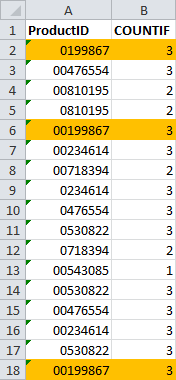
Drag it down, and let’s look at what we get.

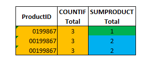
Unfortunately, COUNTIF is doing what we predicted… It is stripping the leading zeros from the numbers, even though they are stored as text. For an example, look at the three rows highlighted in orange. Even though there one is 0199867 and the other two are 00199867, COUNTIF still counts all three together.

Counting Numbers with SUMPRODUCT

Fortunately, there is another way… Most people don’t know, but SUMPRODUCT can do conditional math, much like SUMIF and COUNTIF can! The secret is in a wrapper that turns TRUE and FALSE statements into 1 and 0, respectively. The way the wrapper works is as follows:

=--(TRUE)

Returns 1.

=--(FALSE)

Returns 0.

When we combine it with a SUMPRODUCT function, we can add up only the TRUE statements!

SUMPRODUCT normally takes multiple arrays (you can brush up on SUMPRODUCT syntax here), but we can build our own array by adding a conditional test. In this case, we want to compare column A to the item in the current row. Wrap the conditional in the –() wrapper, and the final SUMPRODUCT formula for cell C2 is as follows:

=SUMPRODUCT(--($A$2:$A$18=A2))

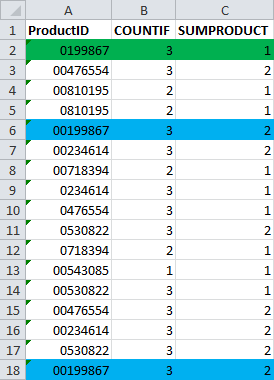
Drag down the formula and let’s look at the result.

And that’s it! That’s what we want! Leading zeros are intact. 0199867 has one entry, and 00199867 has 2. The other entries behave the same way.