Data comes to us in many forms, and often our biggest challenge is translating it from the form it came in into the form we need it in. Date-based data is especially challenging – there are days of the week, weekly totals, months with different numbers of days, and holidays that land on different weekdays each year. This article is part of a series that will help you work with date-based data in Excel to get it into the formats you need.

This tutorial will teach you how to convert weekly summary data into monthly total data by allocating the days in each week to the appropriate month of the year. Let’s dive in!

Examine the Data Set

First off, let’s take a look at our sample data…

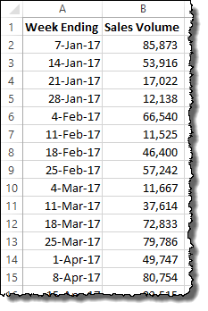
Here we have some pretty standard weekly aggregated sales data. In Column A, we have a date field listing the ending date of each week (Saturday). In Column B we have total sales that occurred in that week.

Throughout this tutorial, we are going to assume that the date provided in your weekly data is the week end. It is still possible to convert week beginning dates and data, but the formulas will need to be changed.

Conversion Assumptions

Since we have only summarized data about each week, there is no way to know exactly what each day’s data was, so you will need to make some assumptions about the daily data. In this tutorial, we’ll assume that each day is average – 1/7th of the week’s total. You could make a different assumption, but it would make the formulas more complicated.

To allocate the correct number of days to each month, we need to build a formula that counts how many days in the week were in the prior month and how many were in the current month. Most weeks will be fully in the current month, so that month will get all of the days. To do this clearly, we are going to create a helper column that helps us calculate the conversion.

Making the Helper Column

In the column next to your weekly data (in our case Column C), create new header and call it “Days In Month” or something similar (the title is just for reference). In the row with the first line of data, type the following formula and press ENTER:

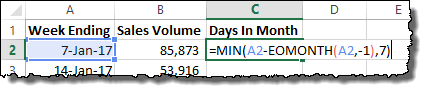
=MIN(A2-EOMONTH(A2,-1),7)

This formula uses the EOMONTH() function. This function provides the date value for the last day of any month, relative to the date provided (The End Of the MONTH). The syntax for the EOMONTH() function is as follows:

EOMONTH(start_date, months)

The start_date is the reference date in Excel date format. The months input is any integer number, positive or negative. If months is zero (0), EOMONTH() provides the last date of the start_date month. If 1, the last day of the next month. If -1, the last day of the prior month, and so on.

In this example, EOMONTH(A2,-1) returns the last day of the month prior to the date in Column A.

The MIN() function just returns the lower of two numbers. In this example, it will calculate (A2 – EOMONTH(A2,-1)) and return whatever is lower – the answer, or the number 7.

In cell C2, The formula is calculating as follows:

MIN(7-Jan-17 - 31-Dec-16 = 7, 7)

In this case, the answers are the same, so the MIN() function returns 7.

Drag the formula down to copy it to all the rows in your data set. When you are finished, you should have a table of data like this:

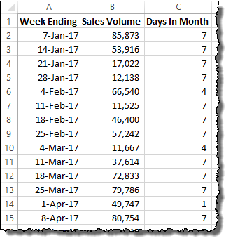
Now, we can add up all the parts of the month to get our monthly totals…

Building the Monthly Total Formula, Part 1

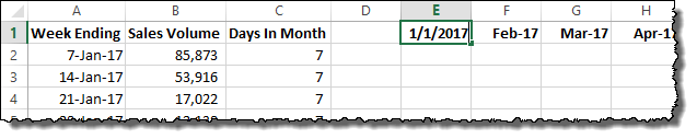
To begin, we need to set up a monthly table.  Next to your data table, build a row of month calendar headings using dates, like shown:

Now, we can begin to capture the portion of the data that falls into each month. To begin, type the following formula in cell E2 and press ENTER:

=SUMPRODUCT((DATE(YEAR($A$2:$A$54),MONTH($A$2:$A$54),1)=DATE(YEAR(E$1),
MONTH(E$1),1))*$C$2:$C$54/7*($B$2:$B$54))

It will look like below, and don’t worry – we’ll walk through what’s going on:

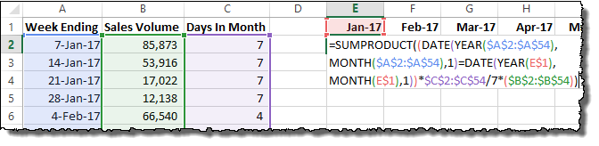
The SUMPRODUCT() function is one big multiplication calculation, but it doing that multiplication for every row in the data table. That’s what the ranges are for ($A$2:$A$54, $B$2:$B$54, and $C$2:$C$54). The part with the DATE() functions is actually comparing two dates and returning a 1 if they are equal and a 0 if they are inequal. Let’s look closer:

(DATE(YEAR($A$2:$A$54),MONTH($A$2:$A$54),1) = DATE(YEAR(E$1),
MONTH(E$1),1))

The first DATE() function is building an Excel date value equal to the month and year of every row in the data table. The second DATE() function is building an Excel date value equal to the month and year of the monthly calendar table.

If they are equal, the SUMPRODUCT() will include the row in the sum. Otherwise, the formula will add zero (excluding them from the sum).

For every row with a date in the current month/year, the rest of the formula is considered:

$C$2:$C$54/7*($B$2:$B$54)

Since Column C is our helper column, it contains the number of days that count in the current month. That number, divided by 7, gives us the fraction of the weekly total to allocate to the current month’s total. We multiply that by the total in Column B, and that’s it!

The SUMPRODUCT() takes the sum of all rows with partial weeks in the current month and adds them together to get the first part of our monthly total.

Building the Monthly Total Formula, Part 2

The first SUMPRODUCT() formula got most of the values we needed, but it left out the partial months that ended mid-week. For example, the week ending February 4, 2017 has 3 days of January in it! To add these days to the total, we need to build another SUMPRODUCT() formula…

Type the following formula in cell E3 and press ENTER:

=SUMPRODUCT((DATE(YEAR($A$2:$A$54),MONTH($A$2:$A$54),1)=DATE(YEAR(E$1),
MONTH(E$1)+1,1))*(7-$C$2:$C$54)/7*($B$2:$B$54))

It will look like below:

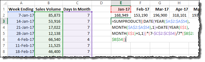
The same logic is at work here as in the previous formula with a few minor tweaks. Instead of comparing dates in Column A to the current month in the monthly calendar table, the formula compares it to the next month in the calendar table:

(DATE(YEAR($A$2:$A$54),MONTH($A$2:$A$54),1)=DATE(YEAR(E$1),
MONTH(E$1)+1,1))

The only difference is a small +1 added to the MONTH() portion of the DATE() formula, highlighted here in red.

The rest of the SUMPRODUCT() formula has also changed:

(7-$C$2:$C$54)/7*($B$2:$B$54)

Instead of using helper Column C as the fraction, we are taking the opposite fraction. Since 7 is our denominator, we start with 7 and subtract the number of days in the (next) month to get the remainder. That fraction of the week is multiplied by the weekly total data and then added to our SUMPRODUCT() total.

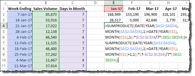
Combining the Monthly Total Formulas

Fortunately, these two SUMPRODUCT() functions can be added together in a single cell to create a total monthly figure for each of the monthly calendar columns. It is as simple as pasting the formulas together with a + in the middle:

=SUMPRODUCT((DATE(YEAR($A$2:$A$54),MONTH($A$2:$A$54),1)=DATE(YEAR(E$1),
MONTH(E$1),1))*$C$2:$C$54/7*($B$2:$B$54)) +
SUMPRODUCT((DATE(YEAR($A$2:$A$54),MONTH($A$2:$A$54),1)=DATE(YEAR(E$1),
MONTH(E$1)+1,1))*(7-$C$2:$C$54)/7*($B$2:$B$54))

It will look like below when completed:

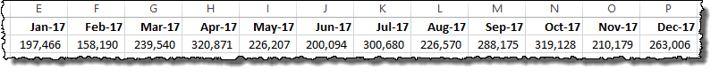
You can drag all three formulas to the right to copy them to each monthly calendar table column. At the end, you should have the same total amount across all your months as you have in your original weekly data set. You can delete the first two rows of the calendar if you prefer, leaving only the combined total monthly sums.

Download the Sample File

The example data used here, as well as all of the formulas discussed is available for download below. You can experiment with the example data in the embed, or download the entire Excel spreadsheet by clicking the download in the bottom right.