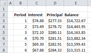Last time, we set out with the goal of building a car loan calculator that could tell us the monthly payment due and how much was owed. It was a great start, but like many of the calculators you can find online, it was missing a lot of details. Today we’re going to take the simple tool we started with and start to add some of those missing features, including a deeper look at the interest payments and the balance over time. Here we go!

Building a Payment Schedule

So far, we have a great little calculation that gives us the monthly payment, but how much of that payment is going towards paying down the debt? How much is being wasted on servicing the interest charges each month? For that, we need to build a table of payments to break it all down. Open the worksheet used last time, or download the example sheet from the last tutorial.

Start a new worksheet or move to an empty one in your workbook and call it “. This table is going to have a lot of data that we don’t need to see on the main sheet.

Label columns for the payment Period, Interest amount, Principal (the amount going to pay down the debt), and the total Balance remaining.

We need a numbered list for all the payment periods. It would be tedious to type them all out, but Excel has a shortcut. Fill in the cells for period 1 and period 2 and select the two cells. Click and hold the lower right corner of the selection box and drag down. When you let go, Excel will automatically guess the series progression and fill in 3, 4, etc. (Quick note, if you had put 1 and 3 in the first boxes, it would have filled in the next as 5, 7, etc. Smart program!)

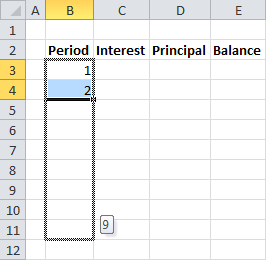
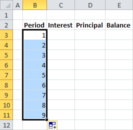
We don’t know exactly how many periods we are going to need to calculate, since someone could change the number in the calculator later, so we need to make it bigger than necessary. It’s unlikely that a car loan will last for  longer than 10 years, so let’s list out 120 periods (one for each month). You can use the drag-down trick to continue the list and Excel will give you a convenient little tool-tip next to the cursor to show you how far down you’ve dragged in the series.

Calculating Interest and Principal Payments

Now, let’s calculate the interest payment for the first period. No payments have been made, so the interest is being charged on the full amount of the loan. We want to multiply the original Loan Amount (C5) by the Interest Rate (C6) and divide by 12 to get the monthly rate. (Remember, APR is for the entire year!)

1. Click on the Interest cell for the first period. In my example spreadsheet, this is C3.
2. Type “=” to tell Excel we are starting a formula.
3. Now, click on the original worksheet tab (called “Car Loan Calculator” the example).
4.  Click C5 (the original loan amount).
5. Type “*” (asterisk) for multiplication.
6. Click C6 (the annual interest rate).
7. Then type “/12” to divide and press ENTER.

The formula should look like this:

='Car Loan Calculator'!C5*'Car Loan Calculator'!C6/12

Excel knows to automatically reference the cells on the other sheet. Fancy!

Now let’s figure out how much there is left to pay towards the principal of the loan. We are going to take the monthly payment from the main calculator and subtract the interest payment we just calculated.

1. Click on the Principal cell for the first period. In my example spreadsheet, this is D3.
2. Type “=” to start the formula.
3. Click on the original worksheet tab (“Car Loan Calculator”).
4. Click on C10 (the monthly payment).
5. Press F4 to lock the reference to the monthly payment.
6. Type “-” for subtraction.
7. Click on the new worksheet tab (“Payment Schedule”).
8. Click on C3 (the interest payment for period 1) and press ENTER.

The formula should look like this:

='Car Loan Calculator'!$C$10-'Payment Schedule'!C3

The $ symbols mean that if this formula is copied around, it won’t change the reference to column C or row 10.

Finally, we need to figure out how much is left in the balance. Since we know how much the original loan was, we can just subtract the principal payment.

1. Click on the Balance cell for the first period. In my example spreadsheet, this is E3.
2. Type “=” to start the formula.
3. Click on the original worksheet tab (“Car Loan Calculator”).
4. Click on C5 (the original loan amount).
5. Type “-” for subtraction.
6. Click on the new worksheet tab (“Payment Schedule”)
7. Click on D3 (the principal payment from period 1) and press ENTER.

The formula should look like this:

='Car Loan Calculator'!C5-'Payment Schedule'!D3

Setting Up Repeating Formulas

We’ve covered the first payment period, but we still need to calculate the rest. So much work! Don’t worry. It gets easier from here. We need to write our calculations in a way that Excel can help us do the work of filling the rest of the table. Let’s set that up in period 2. First, we’ll calculate the interest payment. This time, the balance has been paid down, so we need to pay interest only on what is left from the last period.

1. Click on the Interest cell for the second period. In my example spreadsheet, this is C4.
2. Type “=” to start the formula.
3. Click on E3 (the remaining balance from period 1).
4. Type “*” (asterisk) for multiplication.
5. Click on the original worksheet tab (“Car Loan Calculator”).
6. Click C6 (the annual interest rate).
7. Press F4 to lock the reference to the interest rate.
8. Then type “/12” to divide and press ENTER.

The formula should look like this:

=E3*'Car Loan Calculator'!$C$6/12

Now we need to calculate the remaining principal payment, but wait! We already did this calculation last time! The math is the same, but it’s just on a different interest payment cell. Fortunately, this is where Excel starts to save us time…

1. Select the Principal cell from period 1 (D3).
2. Press CTRL+C to copy the cell formula.
3. Select the Principal cell from period 2 (D4).
4. Press CTRL+V to paste the cell formula in the new cell.

Look at the formula you just pasted. It should look like this:

='Car Loan Calculator'!$C$10-'Payment Schedule'!C4

Look how the reference to C10 stayed the same, but the reference to C3 changed to C4! Smart program!

Now we just need to quickly do the math to find out the remaining balance. This is easy – it’s all on the same page again.

1. Select the Balance cell from period 2 (E4).
2. Type “=” to start the formula.
3. Click E3 (the remaining balance from period 1).
4. Type “-” for subtraction.
5. Click D4 (the principal payment from period 2) and press ENTER.

The formula should look like this:

=E3-D4

Expanding the Payment Schedule Table

Believe it or not, now we’re in business! Remember that drag down trick I showed you earlier? We’re going to use it to finish up this work for us.

Select the interest, principal, and balance cells from period 2 (C4, D4, and E4).

Click and hold the lower right corner of the selection box and drag down all the way to the 120th period.

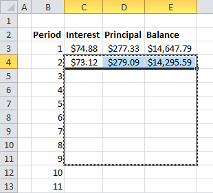
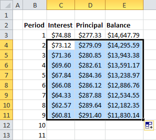
How’s that for making short work of the formulas? Don’t worry that the calculations go negative towards the end. We’re only going to use the ones we need (to get to zero) and we’ll ignore the rest. If you see a series of hash symbols (#######) instead of numbers at the bottom of the table, don’t worry. The formulas are there, but the columns need to be resized.

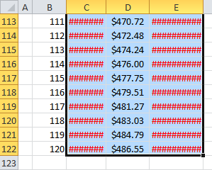
Move your cursor over the vertical line that separates the labels for columns E and F and double-click to automatically resize the column to fit. Do the same between columns C and D.

Calculating Total Interest

We finally have a complete payment schedule table! As a final step, let’s sum all the interest paid throughout the life of the loan.

On the original “Car Loan Calculator” tab, add a line underneath Total Cost that reads Interest Paid (B12 in my example). We are going to sum the interest payments for all the periods in the loan but leave out the extra ones at the bottom using a clever SUMIF function. (If you want to review how SUMIF works, you can click here).

1. Click C12 (the output cell for interest paid).
2. Type “=SUMIF(” to start a SUMIF function.
3. Click on the new worksheet tab (“Payment Schedule”).
4. Click on the column label for column B (the payment period column).
5. Type “,”<=”&“.
6. Click on the old worksheet tab (“Car Loan Calculator”).
7. Click C7 (the term of the loan).
8. Type “,“.
9. Click on the new worksheet tab (“Payment Schedule”).
10. Click on the column label for column C (the interest payment column).
11. Press ENTER. (Excel will auto-complete the formula with the closing parenthesis).

The formula should look like this:

=SUMIF('Payment Schedule'!B:B,"<="&'Car Loan Calculator'!C7,'Payment Schedule'!C:C)

Car Loan Calculator Example

Congrats! Now the calculator has a complete payment table and a way to calculate total interest paid. This goes a long way towards showing  the downside of a loan with a long term. The payments may be low, but the amount of interest you pay skyrockets! You can play around with different loan terms and interest rates right here in the example spreadsheet. If you want to download it to compare to your own, click on the green Excel icon in the lower right.

The payment table is going to come in handy later as we continue to add features to this tool. Come back again for Part 3 to learn how to build a data table that can explore different interest rates and loan terms at the same time!