When you are looking at a large list of numerical data, it’s useful to find maximums and minimums. You can always sort the list to find the largest totals, but if you can’t modify the data (or want to sort by some other rule, like alphabetical), you might need another way to find the max or min. Conditional Formatting in Excel lets you set rules for highlighting values just like you would when using IF statements. Let’s walk through an example using quarterly sales data…

Examine the Data

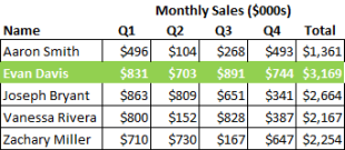
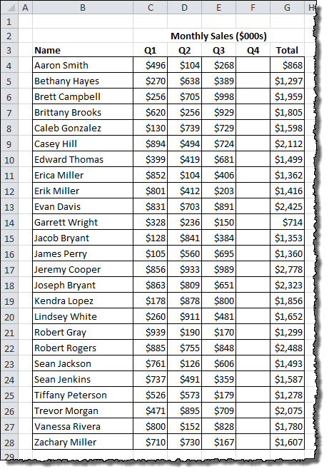
First let’s look at the data… It’s fairly straightforward – just alphabetically sorted employees with their sales figures by quarter. There is already a total column at the end, which we’ll be able to use for our highlighting experiment.

Add Conditional Formatting

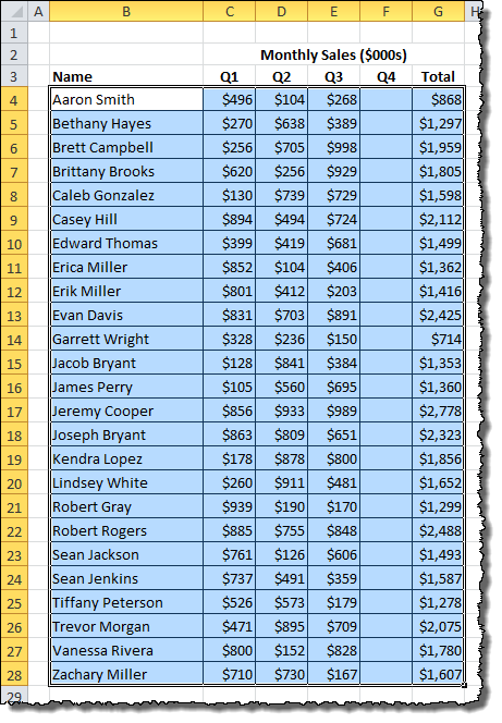
First, select the cells you want to be affected by the formatting rule.

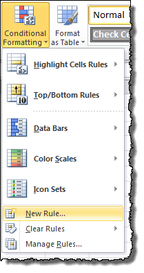
On the Home menu tab, Click on Conditional Formatting under the Styles menu. From the drop-down menu, choose New Rule…

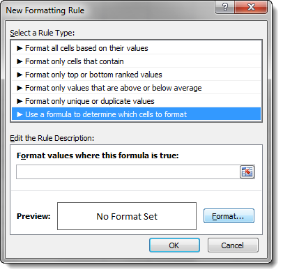
Conditional Formatting gives you a lot of built-in options for formatting rules, but we’re going to write our own. Choose Use a formula to determine which cells to format and click Format to set up how your want your highlight to look. I set my text to bold and my background to green.

Click OK when you’re done to return to the Edit Formatting Rule menu.

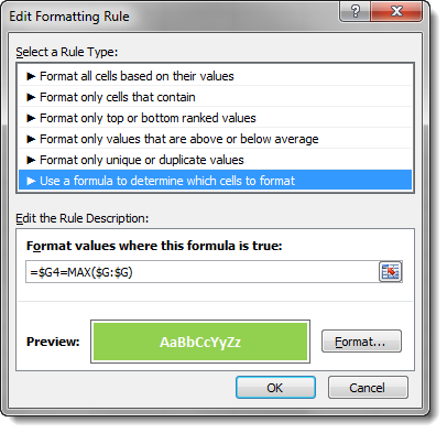
We need to define a conditional rule that will compare the largest value in the total column to each row. Excel has a MAX function that returns the largest value in the range you specify. We want to compare this to the Total cell in the same row as each cell we are testing.

Conditional Formatting assumes that the testing rule is starting in the top left corner of the selection. It will change the cell references relative to each cell it tests, unless you lock them out. Since we want to keep our comparison restricted to the Total column, we’ll lock the column references in the formula. The final equation is:

=$G4=MAX($G:$G)

You may need to type/paste it directly into the field, as Excel tries to “help” fill out the formula if you click around.

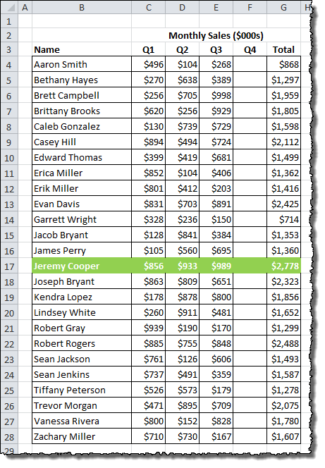
Click OK when the formula is entered. Done correctly, here’s how your data set will look:

Test the Conditional Formatting

It works! But we want to make sure the formatting will update when the data changes… Let’s add Quarter 4 data into column F and see what happens.

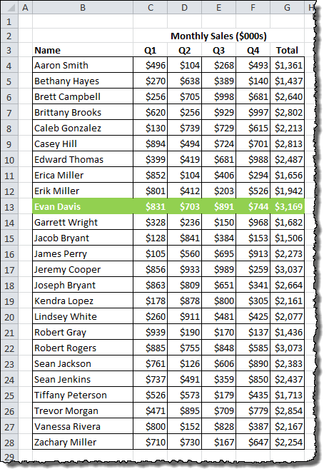
Sure enough, the highlighted row changes to the new maximum!

Conditional Formatting Highlight Example

Below is the example file used in this exercise. You can look at the data before the conditional formatting in the first sheet and after in the second. You can also download the example file by clicking the Excel icon in the lower right.