Quick Navigation
 Dates don’t always get imported into Excel in a nice, clean, ready to use format. When they don’t, it can be a huge hassle – un-formatted dates can’t be added or subtracted, or even filtered or sorted easily. It is usually best to convert them to the standard Excel date format. Excel has an entire array of functions you can use to work with them once you do (you can learn about them here). Excel’s string manipulation functions can help you convert date text to the Excel date format. Let’s walk through an example…
Decimal Separated Date Example
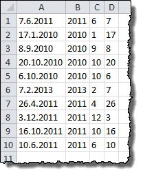
Assume we’ve imported a series of dates that are separated by decimals. For example, 29.09.2013 represents September 29, 2013. Here is a list of examples:

We are going to use the LEFT, RIGHT, and MID functions along with the FIND function to separate out different parts of the date. Then, we can use the DATE function to stitch them together into Excel’s date format. The DATE function takes the year, month, and then day as inputs, so we’ll start by extracting the year…
Extracting the Year from Text
In our example, the year is always the last 4 characters in the date string, so it is easy to recover using the RIGHT function. The syntax is as follows:
=RIGHT(text, [num_chars])
Using the RIGHT function, we can specify the cell the date is in and then 4 to select the first 4 characters from the right. The formula for the first row in our example will be as follows:
=RIGHT(A1,4)
Extracting the Month from Text
The month is most complicated to pull out of the text string. We know that it will be in between two periods, but we don’t know where those periods will occur since months and days can have one or two characters each. This is where FIND comes in. We can use it to locate each decimal point and then guide a MID function to the correct location.
The FIND function has the following syntax:
=FIND(find_text, within_text, [start_num])
To find the first decimal, the basic function looks like this:
=FIND(".",A1)
To find the second decimal, we can nest two FIND functions together. The second FIND (plus 1), tells the first one where to start looking (just past the first decimal):
=FIND(".",A1,FIND(".",A1)+1)
We can use these functions to construct a MID function. MID has the following syntax:
=MID(text, start_num, num_chars)
We give MID A1 as it’s text input. The start_num input will be the first FIND statement. To get the number of characters, we need to know the distance between the first and second decimal.
We can do this by subtracting the first decimal location (the first FIND function) from the second. The final MID function looks like this:
=MID(A1,FIND(".",A1)+1,FIND(".",A1,FIND(".",A1)+1)-FIND(".",A1)-1)
We subtract one more from the difference in the num_chars because the FIND function finds the decimal and not the first character past it, so we actually need to subtract (FIND+1) from the second FIND.
Extracting the Day from Text
The day is similarly easy to extract to the year, only we use the LEFT function instead. The only difference is that we need to FIND the first decimal to determine how many characters we need. The syntax for LEFT is as follows:
=LEFT(text, [num_chars])
Using the first FIND formula from above, the extraction formula for the first row in our example is as follows:
=LEFT(A1,FIND(".",A1)-1)
Stitching the Year, Month, and Day into a DATE
Now that we have the individual components, we can stitch them together. The DATE function syntax is as follows:
=DATE(year, month, day)
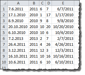
If you’ve been building out the components, your spreadsheet might look something like this:
If so, you can build the DATE function to look at the formulas you have already made. The DATE function for the first row will look like this:
=DATE(B1,C1,D1)
However, if you need all the work to happen in one cell, you can combine all the previous formulas to create a monster:
=DATE(RIGHT(A1,4),
      MID(A1,FIND(".",A1)+1,
          FIND(".",A1,FIND(".",A1)+1)-FIND(".",A1)-1),
      LEFT(A1,FIND(".",A1)-1))
The end result in either case is a beautifully formatted Excel date:
I have found that it may be a little easier to use the “Text to columns” tool instead of having to write all of those formulas to split up the information. After separating them by the decimal place, you can use a simple “Concatenate” formula to put them back together in the correct order and format. Then you would copy and paste the new column as values and then format as a date.
Hi Samantha,
I agree – Text to Columns is another great resource for handling this type of problem. I like Excel’s string manipulation tools because you can use them to find and separate much more complicated strings too. Dates are a simpler case, and it’s good to have multiple approaches to solve it!
Andrew
How to parse a column of dates that are inconsistent: some are 9-10-77 some are 9/10/77, some are Sept 10, 1977, etc. and even 9/77. Standardizing multiple formats such as this requires “different” formulas.
I think the easiest way is to highlight all the cells and use find/replace. Put find as “.” and replace as “/”. Then format the cells as dates.
Genius. The formula gave me some wacky results – some were right and others were just odd, two of the fields would be right and the year would be totally wrong.
Thanks, its just wonderful.
I found that it was actually easier just to do a simple find & replace the decimals with backslashes and then excel will recognize it as dates! 🙂
Simplicity wins! But how did the folks who made all those formulas not think of that? So much faster!
Personally I wouldn’t bother with the complicated formulas. I just used the find and replace, it worked a treat and was far simpler.